1. Characteristics
Scalar_XY is a set of three modules for:
Generation of 2D (xy-axis) light source.
Generation of 2D (xy-axis) masks and diffractive optical elements.
Propagation of light, determination of parameters, and other functions.
Drawing sources, masks and fields.
These modules are named: scalar_fields_XY.py, scalar_sources_XY.py, and scalar_masks_XY.py.
Each module present a main class:
Scalar_field_XY
Scalar_masks_XY
Scalar_sources_XY
The main attributes for these classes are the following:
self.x (numpy.array): linear array with equidistant positions. The number of data is preferibly :math:
2^n.self.y (numpy.array): linear array with equidistant positions. The number of data is preferibly :math:
2^n.self.wavelength (float): wavelength of the incident field.
self.u (numpy.array): complex field with size 2D x.y
We can also find these atributes: * self.X (numpy.array): equal size to x * y. complex field * self.Y (numpy.array): equal size to x * y. complex field * self.quality (float): quality of RS algorithm. Valid for values > 1. * self.info (str): description of data. * self.type (str): Class of the field. * self.date (str): date when performed.
The dimensional magnitudes are related to microns: micron = 1.
Creating an instance
[1]:
from diffractio import sp, nm, plt, np, mm, degrees, um
from diffractio.scalar_fields_XY import Scalar_field_XY
from diffractio.scalar_sources_XY import Scalar_source_XY
from diffractio.scalar_masks_XY import Scalar_mask_XY
Creating a light beam. An instance must be created before starting to operate with light sources. The initialization accepts several arguments.
[2]:
wavelength = 0.5 * um
x0 = np.linspace(-0.25 * mm, 0.25 * mm, 512)
y0 = np.linspace(-0.25 * mm, 0.25 * mm, 512)

u0 = Scalar_source_XY(x=x0, y=y0, wavelength=wavelength, info='u0')
Light sources are defined in the scalar_sources_xy.py module. When the field is initialized, the amplitude of the field is zero. There are many methods that can be used to generate a light source:
plane_wave: Generates a plane wave with a given direction and amplitude
gauss_beam: Generates a gauss beam with a given amplitude, direction, beam-waist and position of beam-waist.
spherical_wave: Generates a spherical wave.
vortex_beam: Generates a vortex beam.
laguerre_beam: Generates a Laguerre beam.
hermite_gauss_beam: Generates a Hermite-Gauss beam.
zernike_beam: Generates aberrated beams using Zernike functions.
bessel_beam: Generates a bessel beam.
plane_waves_several_inclined: Generate several plane waves with different incident angles.
plane_waves_dict: Generate several plane waves with parameters defined in a dictionary.
gauss_beams_several_parallel: Generates a number of parallel gauss beam at different positions.
gauss_beams_several_inclined: Generates a number of gauss beams all placed at the same position but with different incidence angles.
For a more detailed description of each method, refer to the individual documentation of each one.
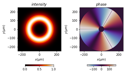
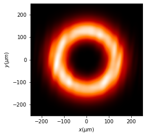
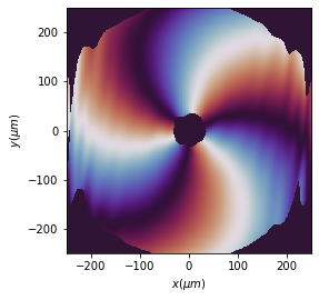
Example: vortex_beam
[3]:
u0.vortex_beam(A=1, r0=(0 * um, 0 * um), w0=100 * um, m=3)
print(u0)
Scalar_source_XY
 - x:  (512,),   y:  (512,),   u:  (512, 512)
 - xmin:       -250.00 um,  xmax:      250.00 um,  Dx:   0.98 um
 - ymin:       -250.00 um,  ymax:      250.00 um,  Dy:   0.98 um
 - Imin:       0.00,     Imax:      1.00
 - phase_min:  -180.00 deg, phase_max: 180.00 deg
 - wavelength: 0.50 um
 - date:       2023-10-07_17_08_05
 - info:       u0
Several ways to show the field are defined: ‘amplitude’, ‘intensity’, ‘field’, ‘phase’, …
[4]:
u0.draw(kind='field')
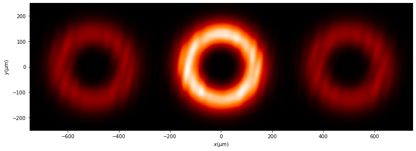
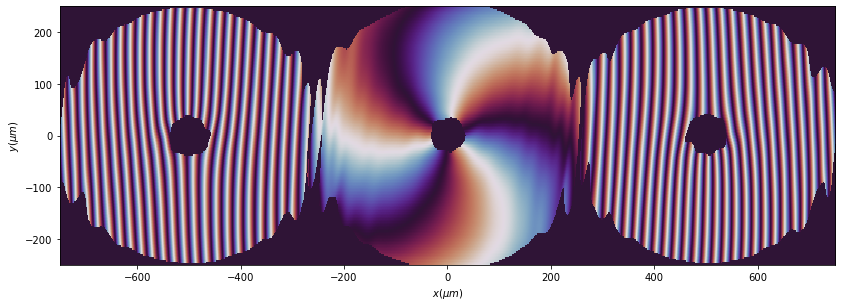
1.1. Basic operations: add to light sources.
[5]:
u1 = Scalar_source_XY(x=x0, y=y0, wavelength=wavelength, info='u1')
u2 = Scalar_source_XY(x=x0, y=y0, wavelength=wavelength, info='u2')

u1.plane_wave(A=1, theta=-.25 * degrees)
u2.plane_wave(A=1, theta=+.25 * degrees)

u_sum = u1 + u2
u_sum.draw(kind='intensity')
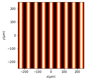
Since we have two plane waves propagating at different angles, an interference effect is produced, shown in the intensity variation of the optical field.
Masks
Masks are defined in the scalar_masks_xy.py module. There are many methods that can be used to generate masks and diffractive optical elements:
set_amplitude, set_phase
binarize, two_levels, gray_scale
a_dataMatrix
area
save_mask
inverse_amplitude, inverse_phase
widen
image
slit, double_slit, square, circle, super_gauss, square_circle, ring, cross
mask_from_function
prism, lens, fresnel_lens
sine_grating, sine_edge_grating ronchi_grating, binary_grating, blazed_grating, forked_grating, grating2D, grating_2D_ajedrez
axicon, biprism_fresnel,
radial_grating, angular_grating, hyperbolic_grating, archimedes_spiral, laguerre_gauss_spiral
hammer
roughness, circle_rough, ring_rough, fresnel_lens_rough,
For a more detailed description of each method, refer to the individual documentation of each one.
Example: Ronchi grating.
[6]:
t0 = Scalar_mask_XY(x=x0, y=y0, wavelength=wavelength, info='t0')
t0.ronchi_grating(x0=0 * um,
                  period=20 * um,
                  fill_factor=0.5,
                  angle=0 * degrees)
t0.draw(kind='intensity')

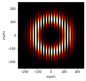
1.2. Basic operations: multiplication of masks and fields
When the light \(u_0\) passes through a mask \(t_0\), the field just after the mask, according to the Thin Element Approximation (TEA), is \(u_1 = t_0 * u_0\). This can be represented in the following way
[7]:
u1 = u0 * t0
u1.draw(kind='intensity')
2. Propagation
Propagation and other actions and parameters of the optical fields are defined in the scalar_field_x.py module. There are several methods of determining the field at a given plane after the mask:
RS: Rayleigh-Sommerfeld propagation at a certain distance
fft: Fast Fourier propagation at the far field.
ifft: Inverse Fast Fourier propagation at the far field.
The field can be stored in the same isntance, generate a new instance, or generate a numpy.array when fast computation is required.
2.1. Near field: Rayleigh-Sommerfeld approach
[8]:
u2 = u1.RS(z=20 * mm, new_field=True)
u2.draw(kind='intensity')
u2.draw(kind='phase')
2.2. Amplification of the field
The Rayleigh-Sommefeld implementation allows an amplification of the field since, sometimes, light diverges:
[9]:
u2 = u1.RS(z=20 * mm, new_field=True, amplification=(3, 1))
u2.draw(kind='intensity', logarithm=False)
fig = plt.gcf()
fig.set_size_inches(13, 6)

u2.draw(kind='phase')
fig = plt.gcf()
fig.set_size_inches(13, 6)
2.3. Reduction of the field
There are some cases where we need to analyze the field in a small area, such as focus of a lens. Then, we can cut and resample the field.
[10]:
wavelength = 0.5 * um
x0 = np.linspace(-0.5 * mm, 0.5 * mm, 1024)
y0 = np.linspace(-0.5 * mm, 0.5 * mm, 1024)

focal = 25 * mm

u0 = Scalar_source_XY(x=x0, y=y0, wavelength=wavelength, info='u0')
u0.plane_wave(A=1, theta=0 * degrees, phi=0 * degrees)

t0 = Scalar_mask_XY(x=x0, y=y0, wavelength=wavelength, info='t0')
t0.lens(r0=(0, 0), radius=(500 * um, 500 * um), focal=(focal, focal))
The field at focal distance results:
[11]:
%%time

u1=t0*u0

u2=u1.RS(z=focal, verbose=False)
u2.normalize();
CPU times: user 1.79 s, sys: 730 ms, total: 2.52 s
Wall time: 2.53 s
[12]:
u2.draw(kind='intensity')
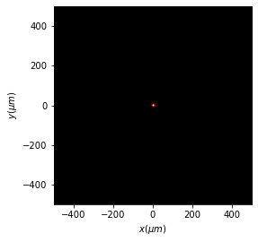
As, the focus cannot be seen properly, we can reduce the field to the desired size.
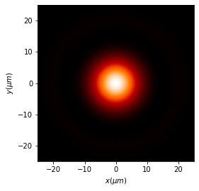
[13]:
u2.cut_resample(x_limits=(-25 * um, 25 * um),
                y_limits=(-25 * um, 25 * um),
                num_points=(512, 512),
                new_field=False)
u2.draw(kind='intensity', logarithm=False)
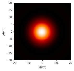
A better possibility is to use CZT algorithm to determine the field at reduced output coordinates.
[14]:
%%time
xout=np.linspace(-20,20,128)
yout=np.linspace(-20,20,128)


u2 = u1.CZT(z=focal, xout=xout, yout=yout)
u2.normalize()
CPU times: user 271 ms, sys: 341 ms, total: 612 ms
Wall time: 614 ms
[15]:
u2.draw(kind='intensity')
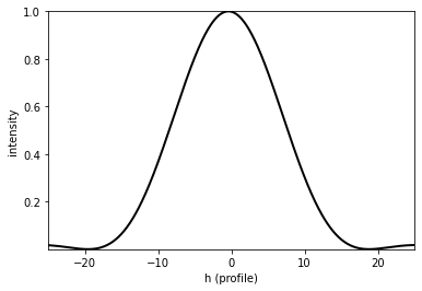
2.4. Focus position and profiles
For focus and other application, the software can detect the position of maximum intensity and determine the profiles in order to a better analysis.
[16]:
x_max, y_max = u2.search_focus(verbose=True)

u2.draw_profile(point1=[-25 * um, x_max],
                point2=[25 * um, x_max],
                npixels=512,
                kind='intensity',
                order=2)
x = -0.283 um, y = -0.283 um