6.2.1. Characteristics
Scalar_XYZ is a set of two modules for:
Generation of 3D masks and diffractive optical elements.
Propagation of light, determination of parameters, and other functions.
Drawing sources, masks and fields
For light generation, scalar_sources_XY.py is used.
Warning: This module is not very mature yet.
These modules are named: scalar_fields_XYZ.py,and scalar_masks_XYZ.py.
Each module present a main class:
Scalar_field_XYZ
Scalar_masks_XYZ
The main attributes for these classes are the following:
self.x (numpy.array): linear array with equidistant positions. The number of data is preferibly \(2^n\) .
self.y (numpy.array): linear array with equidistant positions. The number of data is preferibly \(2^n\) .
self.z (numpy.array): linear array with equidistant positions. The number of data is preferibly \(2^n\) .
self.wavelength (float): wavelength of the incident field.
self.u (numpy.array): equal size than x * y * z. complex field.
We can also find these atributes:
self.X (numpy.array): linear 2D array with size x * y * z storing X position.
self.Y (numpy.array): linear 2D array with size x * y * z storing Y position.
self.Z (numpy.array): linear 2D array with size x * y * z storing Z position.
self.quality (float): quality of RS algorithm. Valid for values > 1.
self.info (str): description of data.
self.fast (bool): If True, Rayleigh-Sommerfeld computations are performed using Fresnel approximation.
self.type (str): Class of the field.
self.date (str): date when performed.
The dimensional magnitudes are related to microns: micron = 1.
[2]:
from diffractio import degrees, eps, mm, no_date, np, plt, um
from diffractio.scalar_fields_XYZ import Scalar_field_XYZ
from diffractio.scalar_masks_XY import Scalar_mask_XY
from diffractio.scalar_masks_XYZ import Scalar_mask_XYZ
from diffractio.scalar_sources_XY import Scalar_source_XY
6.2.1.1. save_load
[3]:
length = 100 * um
numdata = 16  # 256
x0 = np.linspace(-length / 2, length / 2, numdata)
y0 = np.linspace(-length / 2, length / 2, numdata)
z0 = np.linspace(-length / 2, length / 2, numdata)
wavelength = 0.5 * um
filename = 'save_load_xyz.npz'

t1 = Scalar_field_XYZ(x=x0, y=y0, z=z0, wavelength=wavelength)

t1.u = np.ones_like(t1.u)
t1.save_data(filename=filename, add_name='')
[4]:
t2 = Scalar_field_XYZ(x=None, y=None, z=None, wavelength=None)
t2.load_data(filename=filename, verbose=False)
6.2.1.2. clear_field
[5]:
length = 100 * um
numdata = 32  # 256
x0 = np.linspace(-length / 2, length / 2, numdata)
y0 = np.linspace(-length / 2, length / 2, numdata)
z0 = np.linspace(-length / 2, length / 2, numdata)
wavelength = 0.5 * um

u0 = Scalar_field_XYZ(x=x0, y=y0, z=z0, wavelength=wavelength)
u0.u = np.ones_like(u0.u)
print(u0.u.max())

u0.clear_field()
print(u0.u.max())
(1+0j)
0j
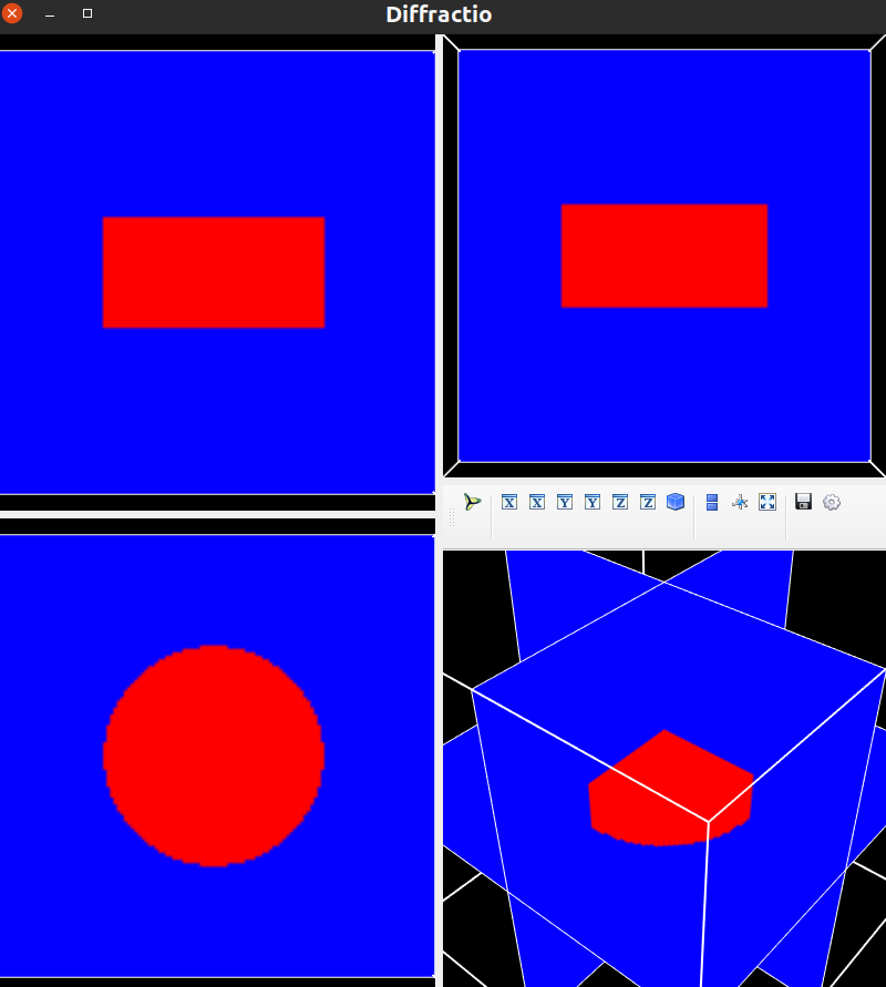
6.2.1.3. show_index_refraccion
[5]:
length = 150 * um

x0 = np.linspace(-length / 2, length / 2, 128)
y0 = np.linspace(-length / 2, length / 2, 128)
z0 = np.linspace(-length / 2, length / 2, 128)
wavelength = 0.55 * um

t1 = Scalar_mask_XY(x=x0, y=y0, wavelength=wavelength)
t1.circle(r0=(0 * um, 0 * um), radius=(20 * um, 20 * um), angle=0 * degrees)

uxyz = Scalar_mask_XYZ(x=x0,
                       y=y0,
                       z=z0,
                       wavelength=wavelength,
                       n_background=1.,
                       info='')
uxyz.incident_field(t1)
uxyz.cylinder(r0=(0 * um, 0 * um, 0),
              radius=(20 * um, 20 * um),
              length=75 * um,
              refractive_index=1.5,
              axis=(0, 0, 0),
              angle=0 * degrees)
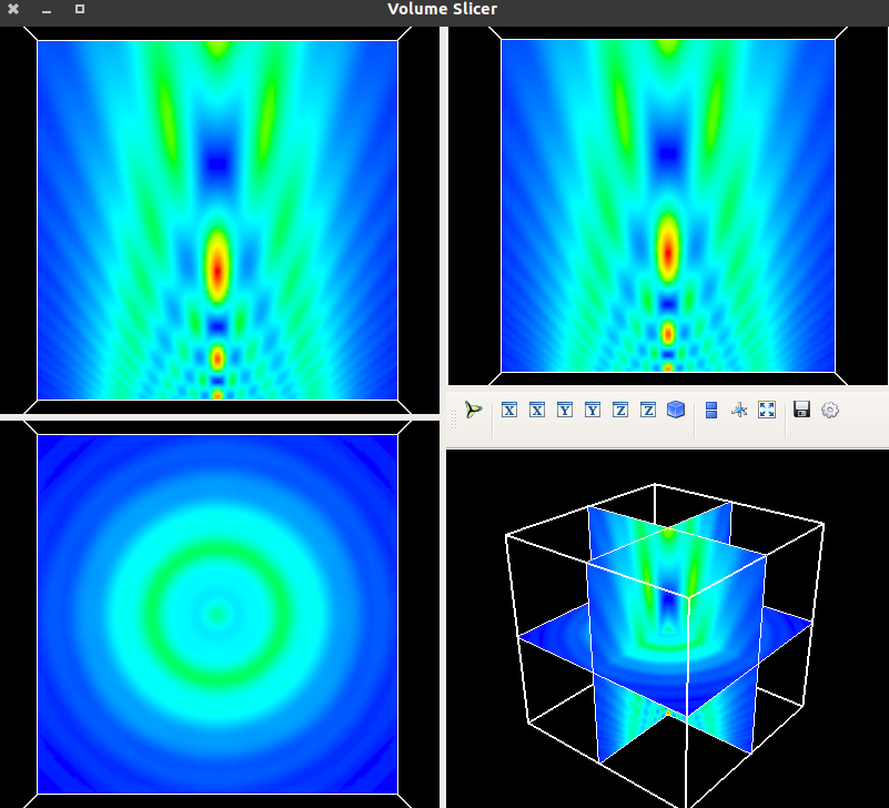
[ ]:
uxyz.draw_volume()
[ ]:
uxyz.draw_refractive_index()
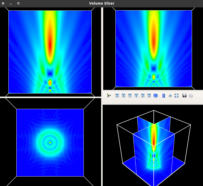
6.2.1.4. RS propagation of a circular aperture
[7]:
length = 100 * um
numdata = 128
x0 = np.linspace(-length / 2, length / 2, numdata)
y0 = np.linspace(-length / 2, length / 2, numdata)
z0 = np.linspace(200 * um, 2 * mm, 128)
wavelength = 0.5 * um

u1 = Scalar_source_XY(x=x0, y=y0, wavelength=wavelength)
u1.gauss_beam(A=1, r0=(0, 0), z0=0, w0=(150 * um, 150 * um))

t1 = Scalar_mask_XY(x=x0, y=y0, wavelength=wavelength)
t1.circle(r0=(0, 0), radius=(25 * um, 25 * um))
t3 = u1 * t1
[8]:
uxyz = Scalar_field_XYZ(x=x0, y=y0, z=z0, wavelength=wavelength)
uxyz.incident_field(t3)
uxyz.RS()
time in RS= 8.317139387130737. num proc= 6
[ ]:
uxyz.draw_XYZ(logarithm=False, normalize='maximum')
6.2.1.5. Rayleigh-Sommerfeld propagation of a gauss beam passing through a Grating
[9]:
length = 500 * um
x0 = np.linspace(-length / 2, length / 2, 128)
y0 = np.linspace(-length / 2, length / 2, 128)
z0 = np.linspace(2 * mm, 7 * mm, 128)
wavelength = 0.6328 * um

u1 = Scalar_source_XY(x=x0, y=y0, wavelength=wavelength)
u1.gauss_beam(A=1, r0=(0, 0), z0=0, w0=(150 * um, 150 * um))

t1 = Scalar_mask_XY(x=x0, y=y0, wavelength=wavelength)
t1.ronchi_grating(x0=0 * um, period=20 * um, angle=0 * degrees)
t2 = Scalar_mask_XY(x=x0, y=y0, wavelength=wavelength)
t2.lens(r0=(0 * um, 0 * um),
        radius=(200 * um, 200 * um),
        focal=(5 * mm, 5 * mm),
        angle=0 * degrees)

t3 = u1 * t1 * t2
[10]:
uxyz = Scalar_field_XYZ(x=x0, y=y0, z=z0, wavelength=wavelength)
uxyz.incident_field(t3)
uxyz.RS()
uxyz.normalize()
time in RS= 9.478154182434082. num proc= 6
[11]:
uxyz.draw_XY(z0=4.5 * mm)
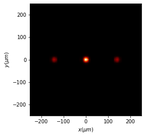
A particular plane, can be passed to scalar_field_XY, and then, it can be drawn.
[12]:
u_xy = uxyz.to_Scalar_field_XY(z0=4.75 * mm, is_class=True, matrix=False)
u_xy.draw(kind='intensity')
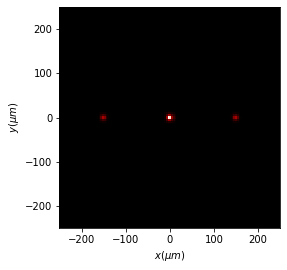
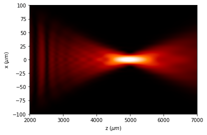
Also, the intensity at the XZ plane can be obtained.
[13]:
uxyz.draw_XZ(y0=0 * mm, logarithm=1e2)
plt.ylim(-100, 100)
<Figure size 432x288 with 0 Axes>
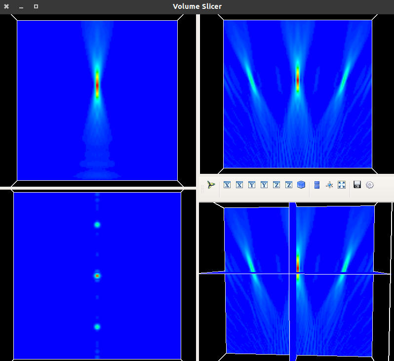
[ ]:
uxyz.draw_XYZ(logarithm=False, normalize='maximum')
6.2.1.6. Video from a XYZ distribution
[6]:
length = 100 * um
numdata = 128  # 256
x0 = np.linspace(-length / 2, length / 2, numdata)
y0 = np.linspace(-length / 2, length / 2, numdata)
z0 = np.linspace(200 * um, 2 * mm, 32)  #128
wavelength = 0.5 * um

u1 = Scalar_source_XY(x=x0, y=y0, wavelength=wavelength)
u1.gauss_beam(A=1, r0=(0, 0), z0=0, w0=(150 * um, 150 * um))

t1 = Scalar_mask_XY(x=x0, y=y0, wavelength=wavelength)
t1.circle(r0=(0, 0), radius=(25 * um, 25 * um))
t3 = u1 * t1
[7]:
uxyz = Scalar_field_XYZ(x=x0, y=y0, z=z0, wavelength=wavelength)
uxyz.incident_field(t3)
uxyz.RS()
uxyz.normalize()
time in RS= 1.6388328075408936. num proc= 6
[8]:
filename = "video_RS"
[9]:
uxyz.video(filename=filename + '_int.mp4', kind='intensity', frame=False)
[11]:
%%HTML
<div align="middle">
      <video width="50%" controls>
            <source src="video_RS_int.mp4" type="video/mp4">
      </video>
</div>
6.2.1.7. benchmark_RS_multiprocessing
[ ]:
x0 = np.linspace(-25 * um, 25 * um, 128)
y0 = np.linspace(-25 * um, 25 * um, 128)
z0 = np.linspace(100 * um, 500 * um, 128)
wavelength = 0.55 * um

t1 = Scalar_mask_XY(x=x0, y=y0, wavelength=wavelength)
t1.circle(r0=(0 * um, 0 * um), radius=(20 * um, 20 * um), angle=0 * degrees)

uxyz = Scalar_mask_XYZ(x=x0,
                       y=y0,
                       z=z0,
                       wavelength=wavelength,
                       n_background=1.,
                       info='')
uxyz.incident_field(t1)
uxyz.sphere(r0=(0 * um, 0 * um, 0 * um),
            radius=(10 * um, 30 * um, 50 * um),
            refractive_index=2,
            angles=(0 * degrees, 0 * degrees, 45 * degrees))
uxyz.u0 = t1
[ ]:
time = uxyz.RS(num_processors=1, verbose=False)
print("time in RS_multiprocessing {}: {} seconds".format(1, time))
[ ]:
time = uxyz.RS(num_processors=4, verbose=False)
print("time in RS_multiprocessing {}: {} seconds".format(4, time))
[ ]:
uxyz.draw_XYZ()
[ ]: