6.1.1. Characteristics
Scalar_X is a set of three modules for:
Generation of 1D (x-axis) light source.
Generation of 1D (x-axis) masks and diffractive optical elements.
Propagation of light, determination of parameters, and other functions.
Drawing sources, masks and fields.
These modules are named: scalar_fields_X.py, scalar_sources_X.py, and scalar_masks_X.py.
Each module present a main class:
Scalar_field_X
Scalar_masks_X
Scalar_sources_X
The main attributes for these classes are the following:
self.x (numpy.array): linear array with equidistant positions. The number of data is preferibly \(2^n\) .
self.wavelength (float): wavelength of the incident field.
self.u (numpy.array): equal size than x. complex field.
We can also find these atributes:
self.quality (float): quality of RS algorithm. Valid for values > 1.
self.info (str): description of data.
self.type (str): Class of the field.
self.date (str): date when performed.
The dimensional magnitudes are related to microns: micron = 1.
Creating an instance
[1]:
from diffractio import sp, plt, np
from diffractio import nm, mm, degrees, um
from diffractio.scalar_fields_X import Scalar_field_X
from diffractio.scalar_sources_X import Scalar_source_X
from diffractio.scalar_masks_X import Scalar_mask_X
Creating a light source.
An instance must be created before starting to operate with light sources. The initialization accepts several arguments.
[2]:
x0 = np.linspace(-0.5 * mm, 0.5 * mm, 1024 * 32)
wavelength = 0.5 * um

u0 = Scalar_source_X(x=x0, wavelength=wavelength, info='u0')
Light sources are defined in the scalar_sources_x.py module. When the field is initialized, the amplitude of the field is zero. There are many methods that can be used to generate a light source:
plane_wave: Generates a plane wave with a given direction and amplitude
gauss_beam: Generates a gauss beam with a given amplitude, direction, beam-waist and position of beam-waist.
spherical_wave: Generates a spherical wave.
plane_waves_several_inclined: Generate several plane waves with different incident angles.
plane_waves_dict: Generate several plane waves with parameters defined in a dictionary.
gauss_beams_several_parallel: Generates a number of parallel gauss beam at different positions.
gauss_beams_several_inclined: Generates a number of gauss beams all placed at the same position but with different incidence angles.
For a more detailed description of each method, refer to the individual documentation of each one.
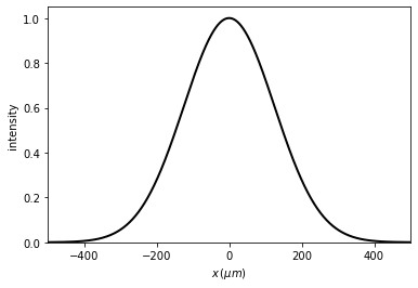
Example: gauss beam.
[3]:
u0.gauss_beam(A=1, w0=250 * um, x0=0, z0=0 * um, theta=0 * degrees)

print(u0)
Scalar_source_X
 - x:  (32768,),   u:  (32768,)
 - xmin:       -500.00 um,  xmax:      500.00 um,  Dx:   0.03 um
 - Imin:       0.00,     Imax:      1.00
 - phase_min:  0.00 deg, phase_max: 0.01 deg
 - wavelength: 0.50 um
 - date:       2023-10-07_17_05_24
 - info:       u0
Several ways to show the field are defined: ‘amplitude’, ‘intensity’, ‘field’, ‘phase’, …
[4]:
u0.draw(kind='intensity')
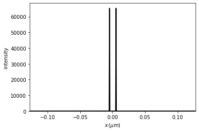
6.1.1.1. Basic operation: add two light sources
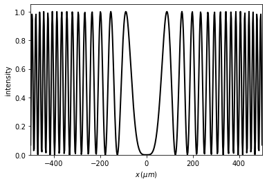
[5]:
x0 = np.linspace(-0.25 * mm, 0.25 * mm, 1024 * 32)
wavelength = 0.5 * um

u1 = Scalar_source_X(x=x0, wavelength=wavelength, info='u1')
u2 = Scalar_source_X(x=x0, wavelength=wavelength, info='u2')

u1.plane_wave(A=1, theta=-1 * degrees)
u2.plane_wave(A=1, theta=+1 * degrees)

u_sum = u1 + u2
u_sum.draw(kind='intensity')
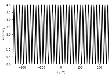
Since we have two plane waves propagating at different angles, an interference effect is produced, shown in the intensity variation of the optical field.
Masks
Masks are defined in the scalar_masks_x.py module. There are many methods that can be used to generate masks and diffractive optical elements:
mask_from_function, mask_from_array
dots
slit, double slit
two_levels, gray_scale
prism, biprism_fresnel, biprism_fresnel_nh
lens, aspheric, fresnel_lens
roughness, dust, dust_different_sizes
sine_grating, ronchi_grating, binary_grating, blazed_grating
chriped_grating, chirped_grating_p, chirped_grating_q
binary_code, binary_code_positions
For a more detailed description of each method, refer to the individual documentation of each one.
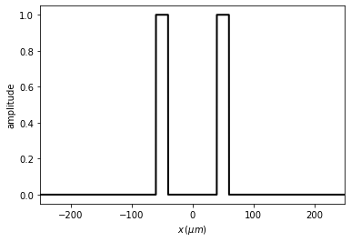
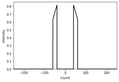
Example: double slit.
[6]:
t0 = Scalar_mask_X(x=x0, wavelength=wavelength, info='t0')
t0.double_slit(x0=0, size=20 * um, separation=100 * um)
t0.draw(kind='amplitude')
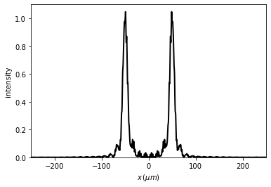
6.1.1.2. Basic operations: multiplication of masks and fields
When the light \(u_0\) passes through a mask \(t_0\), the field just after the mask, according to the Thin Element Approximation (TEA), is \(u_1 = t_0 . u_0\). This can be represented in the following way:
[7]:
u1 = t0 * u0
u1.draw(kind='intensity')
6.1.1.3. Propagation
Propagation and other actions and parameters of the optical fields are defined in the scalar_field_x.py module. There are several methods of determining the field at a given plane after the mask:
RS: Rayleigh-Sommerfeld propagation at a certain distance
fft: Fast Fourier propagation at the far field.
ifft: Inverse Fast Fourier propagation at the far field.
The field can be stored in the same instance, generate a new instance, or generate a numpy.array when fast computation is required.
Other propagation techniques are possible, in the XZ scheme, which is an extension of X scheme.
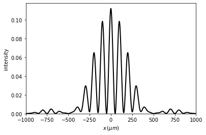
6.1.1.3.1. Near field: Rayleigh-Sommerfeld approach
[8]:
u2 = u1.RS(z=0.5 * mm, new_field=True, verbose=True)
u2.draw(kind='intensity')
Good result: factor 36.57
[9]:
u2 = u1.RS(z=20 * mm, amplification=4, new_field=True, verbose=True)
u2.draw(kind='intensity')
Good result: factor 326.46
Good result: factor 642.94
Good result: factor 4633.98
Good result: factor 33409.94
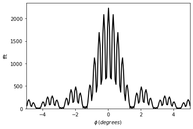
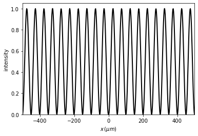
6.1.1.3.2. Far field: Fast Fourier transform
[10]:
u3 = u1.fft(new_field=True, shift=True)
u3.draw(kind='fft', normalize=True)
plt.xlim(-5, 5)
plt.ylim(0)
6.1.1.3.3. Inverse propagation: IFFT
[11]:
x = np.linspace(-500 * um, 500 * um, 512)
wavelength = .5 * um

t1 = Scalar_field_X(x, wavelength)
t1.u = np.sin(2 * np.pi * x / 100)

t2 = t1.fft(z=None,
            shift=True,
            remove0=False,
            matrix=False,
            new_field=True,
            verbose=False)
t2.draw()

t3 = t2.ifft(z=None,
             shift=True,
             remove0=False,
             matrix=False,
             new_field=True,
             verbose=False)
t3.draw()
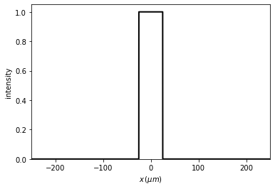
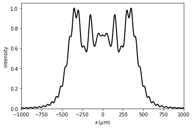
6.1.1.3.4. Amplification of the field
The Rayleigh-Sommefeld implementation allows an amplification of the field since, sometimes, light diverges. Processing time increases approximately linearly with amplification number.
[12]:
wavelength = 0.5 * um
x0 = np.linspace(-0.25 * mm, 0.25 * mm, 1024 * 8)

u0 = Scalar_source_X(x=x0, wavelength=wavelength, info='u0')
u0.spherical_wave(A=1, x0=0, z0=-0.25 * mm)

t0 = Scalar_mask_X(x=x0, wavelength=wavelength, info='t0')
t0.slit(x0=0, size=50 * um)
t0.draw(kind='intensity')

u1 = t0 * u0

t2 = u1.RS(z=5 * mm, amplification=4, verbose=False)
t2.normalize()
t2.draw(kind='intensity')
6.1.1.3.5. Reduction of the field
There are some cases where we need to analyze the field in a small area, such as focus of a lens.
[13]:
focal = 5 * mm
u0 = Scalar_source_X(x=x0, wavelength=wavelength, info='u0')
u0.plane_wave(A=1, theta=0 * degrees)
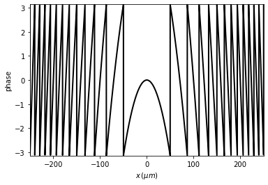
t0 = Scalar_mask_X(x=x0, wavelength=wavelength, info='t0')
t0.lens(x0=0, focal=focal, radius=0)
t0.draw(kind='phase')
[14]:
u1 = t0 * u0

t2 = u1.RS(z=focal, verbose=False)
t2.normalize()
t2.draw(kind='intensity')
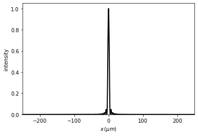
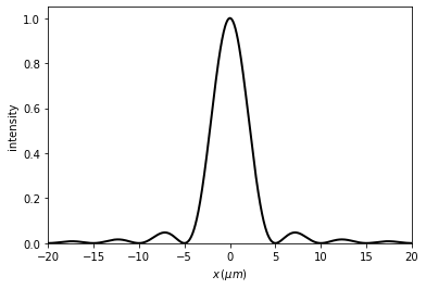
As we cannot see the details, we can use the cut_resample function in order to amplify the focusing zone.
[15]:
t2.cut_resample(x_limits=(-20 * um, 20 * um), num_points=2048, new_field=False)
t2.draw(kind='intensity')
6.1.1.4. Other operations
6.1.1.4.1. Saving and loading data from instance
saving
[16]:
x = np.linspace(-500 * um, 500 * um, 512)
wavelength = .5 * um
filename = 'save_load.npz'

t1 = Scalar_field_X(x, wavelength)
t1.u = np.sin(x**2 / 5000)
t1.draw()

t1.save_data(filename=filename)

loading
[17]:
t2 = Scalar_field_X(x, wavelength)
t2.load_data(filename=filename)
t2.draw()
6.1.1.5. Inserting a mask in other instance
[18]:
x1 = np.linspace(-500 * um, 500 * um, 512)
wavelength = .5 * um
t1 = Scalar_field_X(x1, wavelength)
x2 = np.linspace(-50 * um, 50 * um, 512)
wavelength = .5 * um
t2 = Scalar_field_X(x2, wavelength)
t2.u = np.sin(2 * np.pi * x2 / 50)
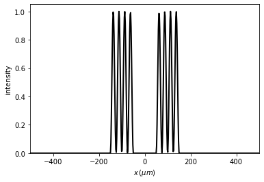
t1.insert_mask(t2, x0_mask1=-100 * um, clean=False, kind_position='center')
t1.insert_mask(t2, x0_mask1=100 * um, clean=False, kind_position='center')
t1.draw()
6.1.1.5.1. Inserting an array of masks in an instance
[19]:
x1 = np.linspace(-750 * um, 750 * um, 2048)
wavelength = .5 * um
t1 = Scalar_field_X(x1, wavelength)
x2 = np.linspace(-50 * um, 50 * um, 2048)
wavelength = .5 * um
t2 = Scalar_field_X(x2, wavelength)
t2.u = np.sin(2 * np.pi * x2 / 50)
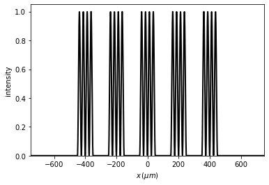
t1.insert_array_masks(t2,
x_pos=[-400, -200, 0, 200, 400],
clean=True,
kind_position='center')
t1.draw()
6.1.1.6. Multiprocessing
For fast computation, several functions are used for generating polychromatic, and extended-size sources:
polychromatic_multiprocessing
extended_source_multiprocessing
extended_polychromatic_source
When the computer present several cores, a signficative increase in speed is obtained.
[20]:
from diffractio.scalar_fields_X import extended_source_multiprocessing
import multiprocessing

num_max_processors = multiprocessing.cpu_count()
A function with only the variable to multiprocess is required:
[21]:
def __experiment_extended_source__(x0):

    x = np.linspace(-333 * um, 333 * um, 1024 * 2)
    wavelength = 0.850 * um
    z0 = -500 * mm
    period = 50 * um
    focal = 5 * mm

    red = Scalar_mask_X(x, wavelength)
    red.ronchi_grating(x0=0 * um, period=period, fill_factor=0.5)

    lens = Scalar_mask_X(x, wavelength)
    lens.lens(x0=0, focal=focal, radius=30 * mm)

    u1 = Scalar_source_X(x, wavelength)
    u1.spherical_wave(A=1., x0=x0, z0=z0, radius=0, normalize=True)
    u2 = u1 * red * lens
    u2.RS(z=focal, new_field=False, verbose=False)

    return u2
[22]:
x0s = np.linspace(-2 * mm, 2 * mm, 1001)
x0_central = 0 * um

intensity, u_s, time_proc = extended_source_multiprocessing(
    __experiment_extended_source__,
    x0s,
    num_processors=num_max_processors,
    verbose=True)
intensity0, u_s0, time_proc0 = extended_source_multiprocessing(
    __experiment_extended_source__, x0_central, num_processors=1, verbose=True)
num_proc: 8, time=1.0968291759490967
num_proc: 1, time=0.006218910217285156
[23]:
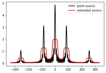
plt.figure()
plt.plot(u_s0.x, np.sqrt(intensity0), 'k', lw=2, label='point source')
plt.plot(u_s[0].x, np.sqrt(intensity), 'r', lw=2, label='extended source')
plt.legend()
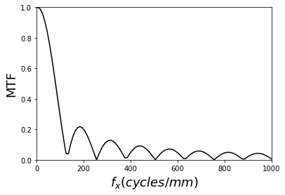
6.1.1.7. Modulation transfer function (MTF)
[24]:
num_data = 1024 * 128
x = np.linspace(-50 * um, 50 * um, num_data)
wavelength = 0.6328 * um

# intensidad de una onda plana
u0 = Scalar_mask_X(x, wavelength)
u0.slit(x0=0, size=8 * um)
u0.draw(kind='intensity')

[25]:
mtf1 = u0.MTF(has_draw=True)
plt.xlim(0, 1000)
plt.ylim(0, 1)