6. Example of light sources

6.1. Creating an instance

An instance must be created before starting to operate with light sources. The initialization accepts several arguments.

[1]:

from diffractio import degrees, mm, np, um
from diffractio.scalar_masks_XY import Scalar_mask_XY
from diffractio.scalar_sources_XY import Scalar_source_XY
from diffractio.vector_masks_XY import Vector_mask_XY
from diffractio.vector_sources_XY import Vector_source_XY

6.2. Procedures to convert a scalar source into a vector source

When a light source is defined using Scalar_source_XY, it can be converted to vectorial using several functions with vector characteristics of the source:

constant_polarization
azimuthal_wave
radial_wave
radial_inverse_wave
azimuthal_inverse_wave
local_polarized_vector_wave
local_polarized_vector_wave_radial
local_polarized_vector_wave_hybrid
spiral_polarized_beam

When the field u in the function is a float number, then it is considered as the amplitude of the wave. Also this functions are masked, with a circular mask, radius=(\(r_x\), \(r_y\)), when \(r_x\) and \(r_y\) >0.

When the parameter results u=1, then the intensity distribution is 1 in both \(E_x\) and \(E_y\) fields.

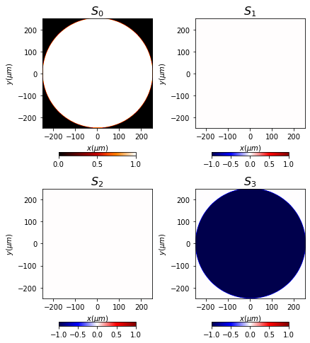
6.2.1. constant polarization wave

[2]:

x0 = np.linspace(-250 * um, 250 * um, 512)
y0 = np.linspace(-250 * um, 250 * um, 512)

wavelength = 0.6328 * um

EM = Vector_source_XY(x0, y0, wavelength)
EM.constant_polarization(u=1, v=(1, 1.j), radius=250 * um)
EM.normalize()
EM.draw('stokes')

../../../_images/source_tutorial_vector_XY_tutorial_vector_sources_XY_5_0.png

[3]:

EM.__draw_ellipses__(logarithm=False,
                     normalize=False,
                     cut_value=None,
                     num_ellipses=(22, 22),
                     amplification=0.75,
                     color_line='r',
                     line_width=.5,
                     draw_arrow=True,
                     head_width=1,
                     ax=False)

../../../_images/source_tutorial_vector_XY_tutorial_vector_sources_XY_6_0.png

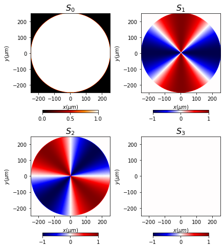
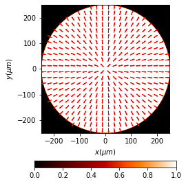
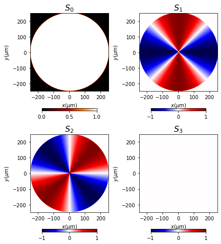
6.2.2. Azimuthal wave

[4]:

x0 = np.linspace(-250 * um, 250 * um, 512)
y0 = np.linspace(-250 * um, 250 * um, 512)

wavelength = 0.6328 * um

EM = Vector_source_XY(x0, y0, wavelength)
EM.azimuthal_wave(u=1, r0=(0, 0), radius=250 * um)
EM.draw('stokes')

../../../_images/source_tutorial_vector_XY_tutorial_vector_sources_XY_8_0.png

[5]:

EM.__draw_ellipses__(logarithm=False,
                     normalize=False,
                     cut_value=None,
                     num_ellipses=(22, 22),
                     amplification=0.5,
                     color_line='r',
                     line_width=1,
                     draw_arrow=True,
                     head_width=3,
                     ax=False)

../../../_images/source_tutorial_vector_XY_tutorial_vector_sources_XY_9_0.png

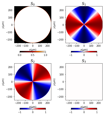
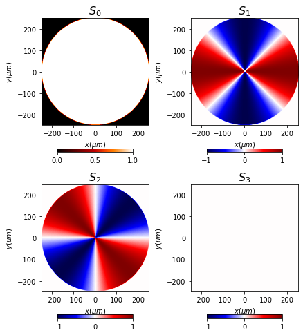
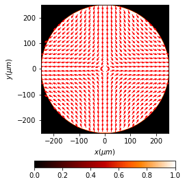
6.2.3. Radial wave

[6]:

x0 = np.linspace(-250 * um, 250 * um, 512)
y0 = np.linspace(-250 * um, 250 * um, 512)

wavelength = 0.6328 * um

EM = Vector_source_XY(x0, y0, wavelength)
EM.radial_wave(u=1, r0=(0, 0), radius=250 * um)
EM.draw('stokes')

../../../_images/source_tutorial_vector_XY_tutorial_vector_sources_XY_11_0.png

[7]:

EM.__draw_ellipses__(logarithm=False,
                     normalize=False,
                     cut_value=None,
                     num_ellipses=(22, 22),
                     amplification=0.5,
                     color_line='r',
                     line_width=1,
                     draw_arrow=True,
                     head_width=3,
                     ax=False)

../../../_images/source_tutorial_vector_XY_tutorial_vector_sources_XY_12_0.png

6.2.4. Azimuthal inverse wave

[8]:

x0 = np.linspace(-250 * um, 250 * um, 512)
y0 = np.linspace(-250 * um, 250 * um, 512)

wavelength = 0.6328 * um

EM = Vector_source_XY(x0, y0, wavelength)
EM.azimuthal_inverse_wave(u=1, r0=(0, 0), radius=250 * um)
EM.draw('stokes')

../../../_images/source_tutorial_vector_XY_tutorial_vector_sources_XY_14_0.png

[9]:

EM.__draw_ellipses__(logarithm=False,
                     normalize=False,
                     cut_value=None,
                     num_ellipses=(22, 22),
                     amplification=0.5,
                     color_line='r',
                     line_width=1,
                     draw_arrow=True,
                     head_width=3,
                     ax=False)

../../../_images/source_tutorial_vector_XY_tutorial_vector_sources_XY_15_0.png

6.2.5. Radial inverse wave

[10]:

x0 = np.linspace(-250 * um, 250 * um, 512)
y0 = np.linspace(-250 * um, 250 * um, 512)

wavelength = 0.6328 * um

EM = Vector_source_XY(x0, y0, wavelength)
EM.radial_inverse_wave(u=1, r0=(0, 0), radius=250 * um)
EM.draw('stokes')

../../../_images/source_tutorial_vector_XY_tutorial_vector_sources_XY_17_0.png

[11]:

EM.__draw_ellipses__(logarithm=False,
                     normalize=False,
                     cut_value=None,
                     num_ellipses=(30, 30),
                     amplification=0.5,
                     color_line='r',
                     line_width=0.5,
                     draw_arrow=True,
                     head_width=5,
                     ax=False)

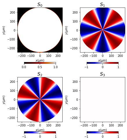
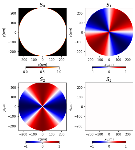
../../../_images/source_tutorial_vector_XY_tutorial_vector_sources_XY_18_0.png

6.2.6. local polarized vector wave

[12]:

x0 = np.linspace(-250 * um, 250 * um, 512)
y0 = np.linspace(-250 * um, 250 * um, 512)

wavelength = 0.6328 * um

EM = Vector_source_XY(x0, y0, wavelength)
EM.local_polarized_vector_wave(u=1,
                               m=2,
                               fi0=np.pi / 2,
                               r0=(0, 0),
                               radius=250 * um)
EM.draw('stokes')

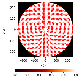
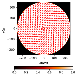
../../../_images/source_tutorial_vector_XY_tutorial_vector_sources_XY_20_0.png

[13]:

EM.__draw_ellipses__(logarithm=False,
                     normalize=False,
                     cut_value=None,
                     num_ellipses=(42, 42),
                     amplification=0.5,
                     color_line='r',
                     line_width=0.5,
                     draw_arrow=True,
                     head_width=3,
                     ax=False)

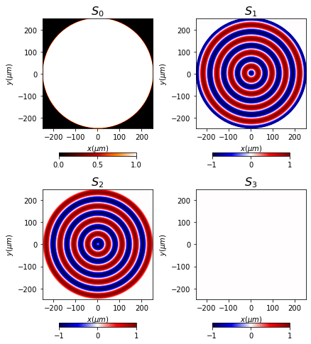
../../../_images/source_tutorial_vector_XY_tutorial_vector_sources_XY_21_0.png

6.2.7. local polarized vector radial beam

[14]:

x0 = np.linspace(-250 * um, 250 * um, 512)
y0 = np.linspace(-250 * um, 250 * um, 512)

wavelength = 0.6328 * um

EM = Vector_source_XY(x0, y0, wavelength)
EM.local_polarized_vector_wave_radial(u=1,
                                      m=2,
                                      fi0=np.pi / 2,
                                      r0=(0, 0),
                                      radius=250 * um)
EM.draw('stokes')

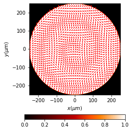
../../../_images/source_tutorial_vector_XY_tutorial_vector_sources_XY_23_0.png

[15]:

EM.__draw_ellipses__(logarithm=False,
                     normalize=False,
                     cut_value=None,
                     num_ellipses=(42, 42),
                     amplification=0.5,
                     color_line='r',
                     line_width=0.5,
                     draw_arrow=True,
                     head_width=3,
                     ax=False)

../../../_images/source_tutorial_vector_XY_tutorial_vector_sources_XY_24_0.png

6.2.8. local polarized vector hybrid beam

[16]:

x0 = np.linspace(-250 * um, 250 * um, 512)
y0 = np.linspace(-250 * um, 250 * um, 512)

wavelength = 0.6328 * um

EM = Vector_source_XY(x0, y0, wavelength)
EM.local_polarized_vector_wave_hybrid(u=1,
                                      n=2,
                                      m=2,
                                      fi0=np.pi / 2,
                                      r0=(0, 0),
                                      radius=250 * um)
EM.draw('stokes')

../../../_images/source_tutorial_vector_XY_tutorial_vector_sources_XY_26_0.png

[17]:

EM.__draw_ellipses__(logarithm=False,
                     normalize=False,
                     cut_value=None,
                     num_ellipses=(42, 42),
                     amplification=0.5,
                     color_line='r',
                     line_width=0.5,
                     draw_arrow=True,
                     head_width=3,
                     ax=False)

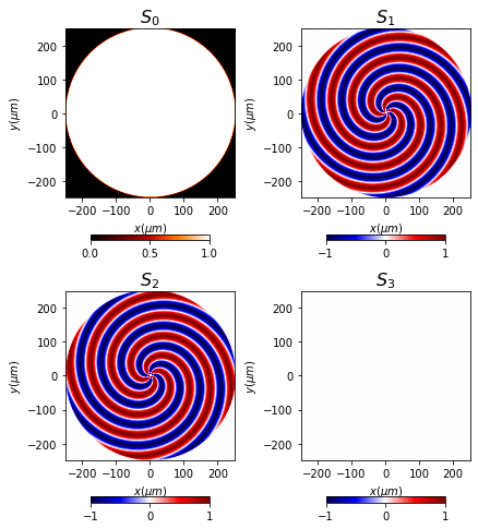
../../../_images/source_tutorial_vector_XY_tutorial_vector_sources_XY_27_0.png

6.2.9. spiral polarized beam

[18]:

x0 = np.linspace(-250 * um, 250 * um, 512)
y0 = np.linspace(-250 * um, 250 * um, 512)

wavelength = 0.6328 * um

EM = Vector_source_XY(x0, y0, wavelength)
EM.spiral_polarized_beam(u=1, r0=(0, 0), alpha=np.pi / 4, radius=250 * um)
EM.draw('stokes')

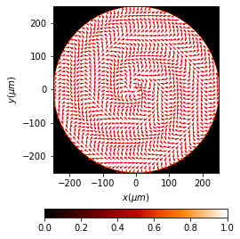
../../../_images/source_tutorial_vector_XY_tutorial_vector_sources_XY_29_0.png

[19]:

EM.__draw_ellipses__(logarithm=False,
                     normalize=False,
                     cut_value=None,
                     num_ellipses=(30, 30),
                     amplification=0.5,
                     color_line='r',
                     line_width=0.5,
                     draw_arrow=True,
                     head_width=5,
                     ax=False)

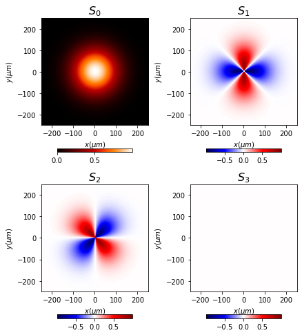
../../../_images/source_tutorial_vector_XY_tutorial_vector_sources_XY_30_0.png

6.3. Generation of a structured beam with polarization

The same functions used previously, can be used to generate vector fields with spatial intensity distribution. In this case, the u parameter is a Scalar_source_XY.

Here, let us see the Gauss beam example.

[20]:

x0 = np.linspace(-250 * um, 250 * um, 512)
y0 = np.linspace(-250 * um, 250 * um, 512)

wavelength = 0.6328 * um

u0 = Scalar_source_XY(x0, y0, wavelength)
u0.gauss_beam(r0=(0, 0),
              w0=(150 * um, 150 * um),
              z0=0 * um,
              A=1,
              theta=0. * degrees,
              phi=0 * degrees)

[21]:

EM = Vector_source_XY(x0, y0, wavelength)
EM.azimuthal_wave(u=u0, r0=(0, 0), radius=250 * um)
EM.draw('stokes')

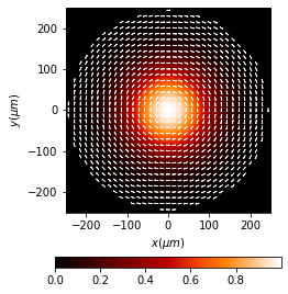
../../../_images/source_tutorial_vector_XY_tutorial_vector_sources_XY_33_0.png

[22]:

EM.draw('ellipses', num_ellipses=(35, 35))

../../../_images/source_tutorial_vector_XY_tutorial_vector_sources_XY_34_0.png

6.4. Vector wave from a scalar source

All these methods to provide vector polarization to a constant wave, can be used for any other scalar source. Then we include in the \(u\) parameters the scalar field:

[23]:

x0 = np.linspace(-250 * um, 250 * um, 512)
y0 = np.linspace(-250 * um, 250 * um, 512)

wavelength = 0.6328 * um

u0 = Scalar_source_XY(x0, y0, wavelength)
u0.plane_wave(A=1, theta=90 * degrees, phi=1 * degrees)

[24]:

EM = Vector_source_XY(x0, y0, wavelength)
EM.azimuthal_wave(u=u0, r0=(0, 0), radius=(200, 200))
EM.__draw_ellipses__(logarithm=False,
                     normalize=False,
                     cut_value=None,
                     num_ellipses=(20, 20),
                     amplification=0.5,
                     color_line='r',
                     line_width=0.5,
                     draw_arrow=True,
                     head_width=5)

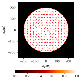
../../../_images/source_tutorial_vector_XY_tutorial_vector_sources_XY_37_0.png

This can also been done, for example to a Gauss beam:

[25]:

x0 = np.linspace(-250 * um, 250 * um, 512)
y0 = np.linspace(-250 * um, 250 * um, 512)

wavelength = 0.6328 * um

u0 = Scalar_source_XY(x0, y0, wavelength)
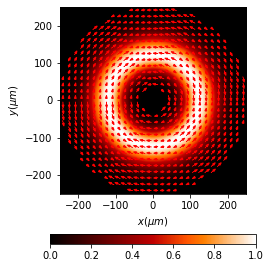
u0.vortex_beam(A=1, r0=(0, 0), w0=100 * um, m=3)

[26]:

EM = Vector_source_XY(x0, y0, wavelength)
EM.azimuthal_wave(u0, r0=(0, 0))
EM.__draw_ellipses__(logarithm=False,
                     normalize=False,
                     cut_value=None,
                     num_ellipses=(30, 30),
                     amplification=0.5,
                     color_line='r',
                     line_width=0.5,
                     draw_arrow=True,
                     head_width=5)

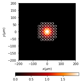
../../../_images/source_tutorial_vector_XY_tutorial_vector_sources_XY_40_0.png

6.5. Gauss Polarization

Since Gauss beams are very used, we have defined the main polarization classes for these beams

[27]:

x0 = np.linspace(-200 * um, 200 * um, 512)
y0 = np.linspace(-200 * um, 200 * um, 512)
wavelength = 0.6328 * um

u1 = Scalar_source_XY(x=x0, y=y0, wavelength=wavelength)
u1.gauss_beam(A=1,
              r0=(0 * um, 0 * um),
              w0=(50 * um, 50 * um),
              z0=0 * um,
              theta=0. * degrees,
              phi=0 * degrees)

EM = Vector_source_XY(x0, y0, wavelength)
EM.constant_polarization(u1, v=(1, 1j))

EM.__draw_ellipses__(logarithm=False,
                     normalize=False,
                     cut_value=None,
                     num_ellipses=(21, 21),
                     amplification=0.75,
                     color_line='w',
                     line_width=.75,
                     draw_arrow=True,
                     head_width=3)

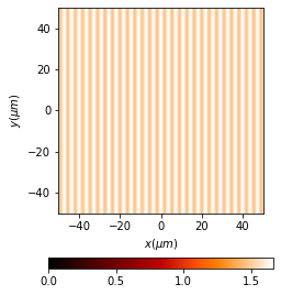
../../../_images/source_tutorial_vector_XY_tutorial_vector_sources_XY_42_0.png

6.6. interferences

Vector fields also interfere. We can sum two vector beams using \(E_M = E_{M1} + E_{M2}\)

[28]:

length = 100 * um
num_data = 512
x0 = np.linspace(-length / 2, length / 2, num_data)
y0 = np.linspace(-length / 2, length / 2, num_data)
wavelength = 0.6328

u1 = Scalar_source_XY(x0, y0, wavelength)
u1.plane_wave(A=1, theta=2 * degrees)

u2 = Scalar_source_XY(x0, y0, wavelength)
u2.plane_wave(A=1, theta=-2 * degrees)

EM1 = Vector_source_XY(x0, y0, wavelength)
EM1.constant_polarization(u=u1, v=[1, 0])

EM2 = Vector_source_XY(x0, y0, wavelength)
EM2.constant_polarization(u=u2, v=[1, 0])

EM = EM1 + EM2
EM.draw(kind='intensity')

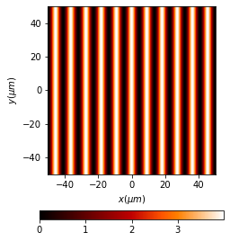
../../../_images/source_tutorial_vector_XY_tutorial_vector_sources_XY_44_0.png

Obviously, when the two beams are ortogonal, no interference is produced:

[29]:

length = 100 * um
num_data = 512
x0 = np.linspace(-length / 2, length / 2, num_data)
y0 = np.linspace(-length / 2, length / 2, num_data)
wavelength = 0.6328

u1 = Scalar_source_XY(x0, y0, wavelength)
u1.plane_wave(A=1, theta=90 * degrees, phi=5 * degrees)

u2 = Scalar_source_XY(x0, y0, wavelength)
u2.plane_wave(A=1, theta=90 * degrees, phi=-5 * degrees)

EM1 = Vector_source_XY(x0, y0, wavelength)
EM1.constant_polarization(u=u1, v=[1, 1j])

EM2 = Vector_source_XY(x0, y0, wavelength)
EM2.constant_polarization(u=u2, v=[1, -1j])

EM = EM1 + EM2
EM.draw(kind='intensity')

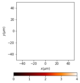
../../../_images/source_tutorial_vector_XY_tutorial_vector_sources_XY_46_0.png

6.6.1. Partial polarization can also be possible.

[30]:

length = 100 * um
num_data = 512
x0 = np.linspace(-length / 2, length / 2, num_data)
y0 = np.linspace(-length / 2, length / 2, num_data)
wavelength = 0.6328

u1 = Scalar_source_XY(x0, y0, wavelength)
u1.plane_wave(A=1, theta=5 * degrees)

u2 = Scalar_source_XY(x0, y0, wavelength)
u2.plane_wave(A=1, theta=-5 * degrees)

EM1 = Vector_source_XY(x0, y0, wavelength)
EM1.constant_polarization(u=u1, v=[1, 0])

EM2 = Vector_source_XY(x0, y0, wavelength)
EM2.constant_polarization(u=u2, v=[0.05, .75])

EM = EM1 + EM2
EM.draw(kind='intensity')

intensity = EM.get(kind='intensity')

../../../_images/source_tutorial_vector_XY_tutorial_vector_sources_XY_48_0.png