6.6.3. Interactive visualization of propagation of light in Jupyter notebook

Matplotlib present useful visualization tools for showing the intensity profiles at a distance z in an interactive fashion in jupyter notebooks. Here, we show how to use it.

In the first place, we well determine the intensity distribution XZ for an object.

from diffractio import degrees, mm, plt, um, np
from diffractio.scalar_sources_X import Scalar_source_X
from diffractio.scalar_masks_XZ import Scalar_mask_XZ

from ipywidgets import interactive

# Initial parameters
x0 = np.linspace(-1050 * um, 1050 * um, 1024 * 2)
z0 = np.linspace(-0.125 * um, 4 * mm, 1024 * 4)
wavelength = 0.6238 * um * 10

# Definition of source
u0 = Scalar_source_X(x=x0, wavelength=wavelength)
u0.gauss_beam(A=1, x0=0 * um, z0=0 * um, w0=2000 * um, theta=0 * degrees)

# insert cylinder
u1 = Scalar_mask_XZ(x=x0, z=z0, wavelength=wavelength, n_background=1)

u1.cylinder(r0=(0, 1.25 * mm), radius=(1 * mm, 1 * mm), refractive_index=1.33, angle=0)
u1.draw_refractive_index(scale="scaled", colorbar_kind="horizontal")

# loading the incident field in the simulation
u1.incident_field(u0)

# WPM propagation
u1.WPM(verbose=False)

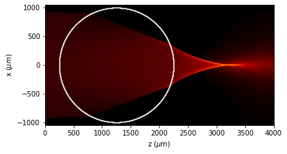
# simple drawing
u1.draw(logarithm=True, scale="scaled", draw_borders=True)

u1.draw_profiles_interactive()

6.6.4. Directly with interactive

%matplotlib widget

Imax = u1.intensity().max()
print(Imax)

75.72461367055705

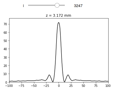
def __interact2__(i):
    plt.plot(u1.x, u1.intensity().transpose()[i], "k")
    plt.title("z = {:2.3f} mm".format(u1.z[i] / 1000))
    plt.ylim(0, Imax)
    plt.xlim(-100 * um, 100 * um)

interactive(__interact2__, i=(0, len(u1.z) - 1, 1))
plt.show()

%matplotlib inline