7.15. Vector Rayleigh-Sommerfeld method

Here we analyze how to obtain the results at the article: H. Ye, C.-W. Qiu, K. Huang, J. Teng, B. Luk’yanchuk, y S. P. Yeo, «Creation of a longitudinally polarized subwavelength hotspot with an ultra-thin planar lens: vectorial Rayleigh–Sommerfeld method», Laser Phys. Lett., vol. 10, n.º 6, p. 065004, jun. 2013.

DOI: 10.1088/1612-2011/10/6/065004 (http://stacks.iop.org/1612-202X/10/i=6/a=065004?key=crossref.890761f053b56d7a9eeb8fc6da4d9b4e).

In this development notebook, we develope Vector Rayleigh-Sommerfeld method. The incident field is an vector field (Ex, Ey) and it is propagated and converted to (Ex,Ey,Ez)

from diffractio import np, sp, plt
from diffractio import nm, um, mm, degrees

from diffractio.vector_sources_XY import Vector_source_XY
from diffractio.scalar_masks_XY import Scalar_mask_XY
from diffractio.scalar_fields_XY import Scalar_field_XY
from diffractio.scalar_sources_XY import Scalar_source_XY

from diffractio.vector_fields_XY import Vector_field_XY

from matplotlib import cm

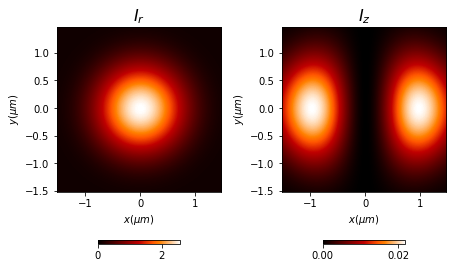
7.15.1. Diffraction by a hole

In Figure 2, a simulation of the electric fields at z=6.5 um from a circular aperture of diameter 5\(\lambda\) is obtained when \(\lambda\) = 0.648 \(\mu\)m.

size = 5 * um
x0 = np.linspace(-size, size, 256)
y0 = np.linspace(-size, size, 256)
wavelength = .640 * um
radius = 5 * wavelength / 2

t = Scalar_mask_XY(x0, y0, wavelength)
t.circle(r0=(0, 0), radius=radius)

E0 = Vector_source_XY(x0, y0, wavelength)
E0.constant_polarization(u=t, v=(1, 0))

%%time
E1=E0.VRS(z=6.5*um, n=1, new_field=True, verbose=False, amplification=(1,1))
E1.cut_resample([-1.5,1.5], [-1.5,1.5])

CPU times: user 357 ms, sys: 40.7 ms, total: 398 ms
Wall time: 396 ms

E1.draw(kind='intensities_rz', logarithm=False)

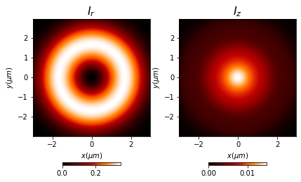
7.15.2. Radial polarized Gaussian beam through a circular aperture

In Figure 3, the propagation of a radially polarized Gaussian beam is performed. The diameter of teh circular aperture is D = 10\(\lambda\), and the beam is FWHM = 6 \(\mu\)m.

size = 6.4 * um
x0 = np.linspace(-size, size, 512)
y0 = np.linspace(-size, size, 512)

wavelength = .640 * um

radius = 10 * wavelength / 2
z_obs = 10 * um
beam_width = 6 * um / (2 * np.sqrt(2))

u0 = Scalar_source_XY(x0, y0, wavelength)
u0.gauss_beam(A=1, r0=(0, 0), w0=beam_width, z0=0)

t0 = Scalar_mask_XY(x0, y0, wavelength)
t0.circle(r0=(0, 0), radius=radius)

t = u0 * t0

E0 = Vector_source_XY(x0, y0, wavelength)
E0.radial_wave(u=t, r0=(0, 0))

E1 = E0.VRS(z=z_obs, n=1, new_field=True)
E1.cut_resample([-3, 3], [-3, 3])

E1.draw('intensities_rz')

Ex, Ey, _ = E1.get('fields', is_matrix=False)
intensity = E1.get('intensity', is_matrix=True)
Ex.u = np.sqrt(intensity)

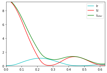
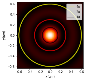
7.15.3. Focusing with a lens a beam with a high \(E_z\) component

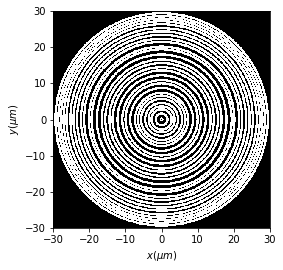
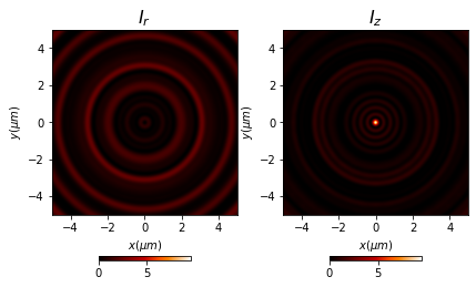
In Figures 4 and 5 a planar lens formed by rings is developed in order to obtain a high \(E_z\) component. The data of the radii are shown in Table 1.

size = 30 * um
x0 = np.linspace(-size, size, 1024)
y0 = np.linspace(-size, size, 1024)

wavelength = .6328 * um
z_obs = 10.32 * um

inner_radius = np.array([
    0.15, 1.3, 2.45, 3.3, 4.25, 5.35, 6.2, 7, 8.35, 9.65, 10.55, 11.9, 13.2,
    14.15, 15.25, 16.2, 17.6, 19.05, 19.8, 21.15, 22, 23.05, 24, 24.95, 26,
    26.8, 27.55, 28.25, 29.05
])

outer_radius = np.array([
    0.5, 1.95, 3.1, 3.95, 4.9, 6, 6.85, 7.65, 9, 10.3, 11.2, 12.55, 13.85,
    14.8, 15.9, 16.85, 18.25, 19.7, 20.45, 21.8, 22.65, 23.7, 24.65, 25.6,
    26.65, 27.45, 28.2, 28.9, 29.7
])

u0 = Scalar_source_XY(x0, y0, wavelength)
u0.plane_wave(A=1)

t0 = Scalar_mask_XY(x0, y0, wavelength)
t0.rings(r0=(0, 0), inner_radius=inner_radius, outer_radius=outer_radius)
t0.pupil()

t = u0 * t0

t0.draw()

E0 = Vector_source_XY(x0, y0, wavelength)
E0.radial_wave(u=t, r0=(0, 0))

E1 = E0.VRS(z=z_obs, n=1, new_field=True)
E1.cut_resample([-5, 5], [-5, 5], num_points=[512, 512])

E1.draw('intensities_rz', logarithm=False)

Ex, Ey, Ez = E1.get('fields', is_matrix=False)

Iz = np.abs(Ez.u)**2
Ir = np.abs(Ex.u)**2 + np.abs(Ey.u)**2

I_total = Iz + Ir

Ex.u = np.sqrt(Ir)
Ey.u = np.sqrt(Iz)

z, I_r, _, _ = Ex.profile([-3, 0], [3, 0], order=2)
z, I_z, _, _ = Ey.profile([-3, 0], [3, 0], order=2)

I_total = I_r + I_z

plt.figure()
plt.plot(z, I_r, 'c', label='Ir')
plt.plot(z, I_z, 'r', label='Iz')
plt.plot(z, I_total, 'g', label='$I_{total}$')
plt.legend()

plt.xlim(0, wavelength)
plt.ylim(ymin=0, ymax=9.25)

Ey.u = Ey.u / Ey.u.max()

Ey.cut_resample([-wavelength, wavelength], [-wavelength, wavelength],
                num_points=[256, 256])

width, _, _, _ = Ey.beam_width_4s()
print("width = {} lambda".format(width / (2 * np.sqrt(2))))

width = 0.4219562175641547 lambda