5. Check power in Rayleigh-Sommerfeld propagation

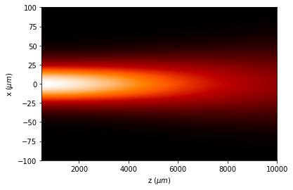
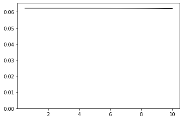
In this example, we verify that the energy of the beam (here we use a Gauss beam) is constant for propagation. We use the XYZ module and Rayleigh-Sommerfeld algorithm.

from diffractio import degrees, eps, mm, no_date, np, um, plt
from diffractio.scalar_fields_XYZ import Scalar_field_XYZ
from diffractio.scalar_masks_XY import Scalar_mask_XY
from diffractio.scalar_masks_XYZ import Scalar_mask_XYZ
from diffractio.scalar_sources_XY import Scalar_source_XY

x0 = np.linspace(-100 * um, 100 * um, 256)
y0 = np.linspace(-100 * um, 100 * um, 256)
z0 = np.linspace(500 * um, 10 * mm, 32)
wavelength = .6328 * um

t1 = Scalar_source_XY(x=x0, y=y0, wavelength=wavelength)
t1.gauss_beam(r0=(0, 0), w0=40 * um, z0=0.0, A=1, theta=0.0, phi=0.0)

uxyz = Scalar_mask_XYZ(x=x0, y=y0, z=z0, wavelength=wavelength)

uxyz.incident_field(u0=t1)

uxyz.RS(verbose=True, num_processors=4)

time in RS= 7.766473054885864. num proc= 4

uxyz.draw_XZ(y0=0)

<Figure size 432x288 with 0 Axes>

intensity = np.abs(uxyz.u)**2

total_energy = intensity.mean(axis=0).mean(axis=0)

plt.plot(z0 / mm, total_energy, 'k')
plt.ylim(ymin=0, ymax=1.05 * total_energy.max())

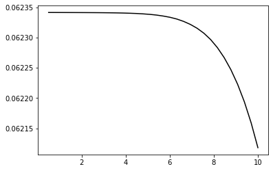
plt.plot(z0 / mm, total_energy, 'k')