5. Chirped Z-transform (CZT)
CZT allows, in a single step, to propagate to a near or far observation plane. IThe main advantage of CZT is that the region of interest and the sampling numbers can be arbitrarily chosen, endowing CZT with superior flexibility, and produces much faster results (acceleration > x100 with respect to RS algorithm) for focusing and far field diffraction patterns.
As the sampling area and pixels can be reduced to the desired observation area, the storage is also greatly reduced.
CZT algorithm allows to have a XY mask and compute in XY, Z, XZ, XYZ schemes, simply defining the output arrays.
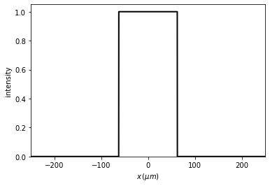
5.1. X Scheme
[1]:
from diffractio import degrees, mm, um, nm
from diffractio import np, plt, sp

from diffractio.scalar_fields_X import Scalar_field_X
from diffractio.scalar_masks_X import Scalar_mask_X
from diffractio.scalar_sources_X import Scalar_source_X

from diffractio.scalar_fields_XZ import Scalar_field_XZ
from diffractio.scalar_fields_Z import Scalar_field_Z
[2]:
size = 250 * um
xin = np.linspace(-size, size, 4096)
wavelength = 550 * nm
z = 2 * mm
[3]:
t0 = Scalar_mask_X(xin, wavelength)
t0.slit(x0=0, size=size / 2)
u0 = Scalar_source_X(xin, wavelength)
u0.plane_wave(A=1)

u1 = t0 * u0
u1.draw()
5.1.1. to just one data
[4]:
xout = 0.
z = 2 * mm
[5]:
%%time
u2 = u1.CZT(z, xout)
print(u2)
[0.63252658+0.60319534j]
CPU times: user 6.8 ms, sys: 0 ns, total: 6.8 ms
Wall time: 5.72 ms
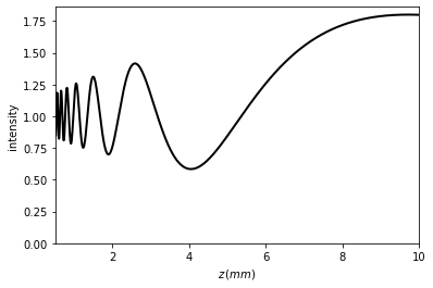
5.1.2. to field_Z
[6]:
xout = 0
z = np.linspace(.5 * mm, 10 * mm, 1024)
[7]:
%%time
u2 = u1.CZT(z, xout, verbose=True)
CPU times: user 3.81 s, sys: 54 ms, total: 3.86 s
Wall time: 3.81 s
[8]:
u2.draw(z_scale='mm')
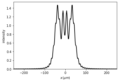
5.1.3. to field_X
[9]:
xout = np.linspace(-size, size, 256)
z = 2 * mm
[10]:
%%time
u2 = u1.CZT(z, xout)
CPU times: user 9.8 ms, sys: 215 µs, total: 10 ms
Wall time: 9.34 ms
[11]:
u2.draw()
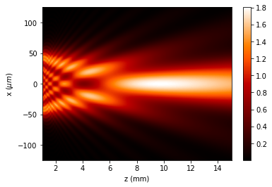
5.1.4. to field_XZ
[12]:
xout = np.linspace(-size / 2, size / 2, 2048)
z = np.linspace(1 * mm, 15 * mm, 128)
[13]:
%%time
u2 = u1.CZT(z, xout, verbose=True)
CPU times: user 1.13 s, sys: 23.2 ms, total: 1.15 s
Wall time: 1.15 s
[14]:
u2.draw(logarithm=0, z_scale='mm')
plt.colorbar()
5.1.5. to data
[18]:
xout = 0
yout = 0.
z = .5 * mm
[19]:
%%time
u2 = u1.CZT(z, xout, yout)
print("{}".format(np.abs(u2)**2))
0.005578354037388983
CPU times: user 65 ms, sys: 23.6 ms, total: 88.6 ms
Wall time: 88.7 ms
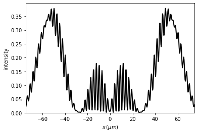
5.1.6. to field_X
[20]:
xout = np.linspace(-size, size, 512)
yout = 0.
z = .5 * mm
[21]:
%%time
u2 = u1.CZT(z, xout, yout)
u2.draw()
CPU times: user 120 ms, sys: 7.92 ms, total: 127 ms
Wall time: 126 ms
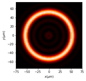
5.1.7. to field_XY
[22]:
xout = np.linspace(-size, size, 256)
yout = np.linspace(-size, size, 256)
z = .25 * mm
[23]:
%%time
u2 = u1.CZT(z, xout, yout)
u2.draw()
CPU times: user 342 ms, sys: 124 ms, total: 465 ms
Wall time: 256 ms
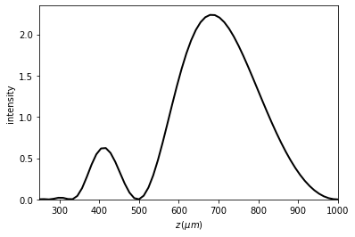
5.1.8. to field_Z
The Z field is computed with a for loop, thus it is a bit slower.
[24]:
xout = -1.
yout = 0.
z = np.linspace(0.25 * mm, 1 * mm, 64)
[25]:
%%time
u2 = u1.CZT(z, xout, yout, verbose=True)
u2.draw()
num x, num y, num z = 1, 1, 64
CPU times: user 3.75 s, sys: 37.4 ms, total: 3.78 s
Wall time: 3.75 s
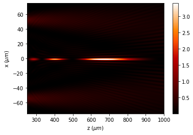
5.1.9. to field_XZ
[26]:
xout = np.linspace(-size, size, 128)
yout = 0.
z = np.linspace(0.25 * mm, 1 * mm, 128)
[27]:
%%time
u2 = u1.CZT(z, xout, yout, verbose=True)
u2.draw()
plt.colorbar()
num x, num y, num z = 128, 1, 128
CPU times: user 7.31 s, sys: 1.9 s, total: 9.22 s
Wall time: 9.22 s
5.1.10. to field_XYZ
[28]:
xout = np.linspace(-size, size, 128)
yout = np.linspace(-size, size, 128)
z = np.linspace(0.25 * mm, 6 * mm, 64)
[29]:
%%time
u2 = u1.CZT(z, xout, yout, verbose=True)
num x, num y, num z = 128, 128, 64
CPU times: user 3.86 s, sys: 815 ms, total: 4.68 s
Wall time: 4.68 s
[30]:
u2.draw_XY(z0=1 * mm)
plt.colorbar()
5.2. CZT for reducing the output size
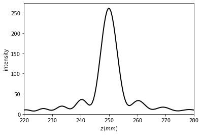
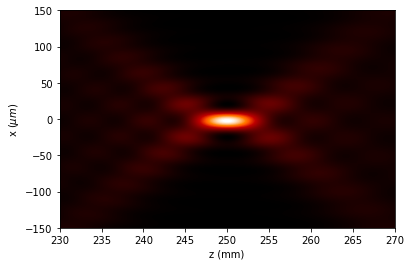
Chirped z-Transform algorithm is specially indicated for cases where the output field is much smaller than the input field, as you can choose the position and sampling of the field. An important example for this is the focusing of a lens.
5.2.1. X scheme
[32]:
size = 3 * mm
xin = np.linspace(-size, size, 4096)
wavelength = 550 * nm
focal = 250 * mm
[33]:
%load_ext autoreload
%autoreload 2
[34]:
t0 = Scalar_mask_X(xin, wavelength)
t0.lens(x0=0, focal=focal)

u0 = Scalar_source_X(xin, wavelength)
u0.plane_wave(A=1)

u1 = t0 * u0
[35]:
xout = 0.
z = np.linspace(focal - 30 * mm, focal + 30 * mm, 128)
[36]:
%%time
u2 = u1.CZT(z, xout, verbose=True)
u2.draw(z_scale='mm')
CPU times: user 591 ms, sys: 4.43 ms, total: 595 ms
Wall time: 596 ms
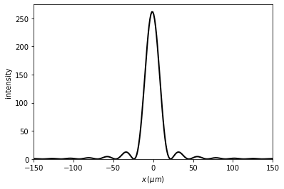
[37]:
xout = np.linspace(-150 * um, 150 * um, 256)
z = focal
[38]:
%%time
u2 = u1.CZT(focal, xout)
u2.draw()
CPU times: user 28.9 ms, sys: 168 µs, total: 29.1 ms
Wall time: 28.4 ms
[39]:
xout = np.linspace(-150 * um, 150 * um, 128)
z = np.linspace(focal - 20 * mm, focal + 20 * mm, 128)
[40]:
%%time
u2 = u1.CZT(z, xout, verbose=True)
u2.draw(logarithm=0, z_scale='mm')
CPU times: user 1.17 s, sys: 2.44 ms, total: 1.17 s
Wall time: 1.16 s
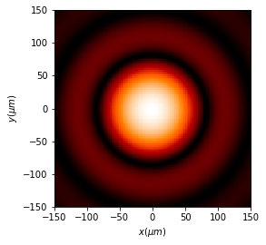
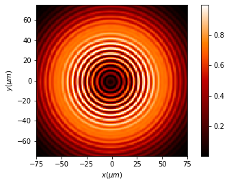
5.2.2. XY scheme
[41]:
size = 2 * mm
xin = np.linspace(-size, size, 512)
yin = np.linspace(-size, size, 512)
wavelength = 550 * nm
focal = 500 * mm
[42]:
t0 = Scalar_mask_XY(xin, yin, wavelength)
t0.lens(r0=(0, 0), focal=focal, radius=0)
t0.pupil()

u0 = Scalar_source_XY(xin, yin, wavelength)
u0.plane_wave(A=1)

u1 = t0 * u0
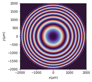
[43]:
xout = np.linspace(-150 * um, 150 * um, 128)
yout = np.linspace(-150 * um, 150 * um, 128)
z = focal
[44]:
%%time
u2 = u1.CZT(z, xout, yout, verbose=True)
u2.draw(logarithm=1e-1)
num x, num y, num z = 128, 128, 1
CPU times: user 408 ms, sys: 279 ms, total: 688 ms
Wall time: 336 ms