1. Fast Fourier Transform (FFT)
Fast Fourier Transform (FFT) is used to determine the field at a distance far away from the mask,
\[z\gg\frac{\pi}{\lambda}\left(\xi^{2}+\eta^{2}\right)_{\max},\]
where \(\xi\) and \(\eta\) are the locations of the mask. The field can be computed using the following integral (in 2D):
\[E(x,y,z)=\frac{e^{ik(z+\frac{x^{2}+y^{2}}{2z})}}{i\lambda z}\iint E_{0}(\xi,\eta)e^{-i\frac{k}{z}(x\xi+y\eta)}d\xi d\eta,\]
which can be computed as a FFT:
\[E(x,y,z)=\frac{e^{ik(z+\frac{x^{2}+y^{2}}{2z})}}{i\lambda z}TF\left[E_{0}(\xi,\eta)\right].\]
[1]:
from diffractio import sp, nm, plt, np, mm, degrees, um
from diffractio.scalar_fields_X import Scalar_field_X
from diffractio.scalar_sources_X import Scalar_source_X
from diffractio.scalar_masks_X import Scalar_mask_X
1.1. X Scheme
[2]:
x0 = np.linspace(-50 * um, 50 * um, 1024 * 32)
wavelength = .5 * um
[3]:
# plane wave
u0 = Scalar_source_X(x=x0, wavelength=wavelength)
u0.plane_wave(A=1, theta=0)
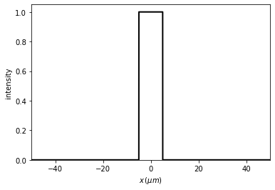
# slit
t0 = Scalar_mask_X(x=x0, wavelength=wavelength)
t0.slit(x0=0, size=10 * um)
t0.draw()
u1 = u0 * t0
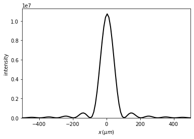
[4]:
u2 = u1.fft(z=2 * mm, remove0=False, new_field=True)
u2.draw(kind='intensity', logarithm=False, normalize=True)
plt.xlim(-500, 500)
plt.ylim(bottom=0)
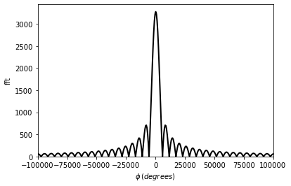
[5]:
u3 = u1.fft(z=2 * mm, remove0=False, new_field=True)
u3.draw(kind='fft', logarithm=False, normalize=True)
plt.xlim(-1e5, 1e5)
plt.ylim(bottom=0)
Fast Fourier Transform using Rayleigh-Sommerfeld (near field) and a lens
Now, let us determine the field at the Fourier plane of the lens.
[6]:
x = np.linspace(-100 * um, 100 * um, 4096)
wavelength = .5 * um
focal = .25 * mm
u0 = Scalar_source_X(x=x0, wavelength=wavelength, info='u0')
u0.plane_wave(A=1, theta=0 * degrees)
t0 = Scalar_mask_X(x=x0, wavelength=wavelength)
t0.slit(x0=0, size=10 * um)
t0.draw()
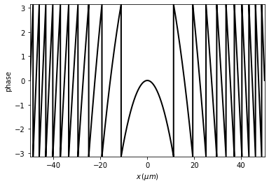
t1 = Scalar_mask_X(x=x0, wavelength=wavelength, info='t0')
t1.lens(x0=0, radius=500, focal=focal)
t1.draw(kind='phase')

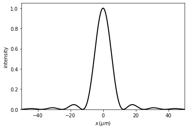
[7]:
u1 = t0 * t1 * u0

t2 = u1.RS(z=focal, verbose=False)
t2.normalize()
t2.draw(kind='intensity')
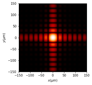
1.2. XY Scheme
[8]:
from diffractio.scalar_sources_XY import Scalar_source_XY
from diffractio.scalar_masks_XY import Scalar_mask_XY
[9]:
x0 = np.linspace(-150 * um, 150 * um, 1024)
y0 = np.linspace(-150 * um, 150 * um, 1024)
wavelength = .5 * um
[10]:
# plane wave
u0 = Scalar_source_XY(x=x0, y=y0, wavelength=wavelength)
u0.plane_wave(A=1, theta=0)
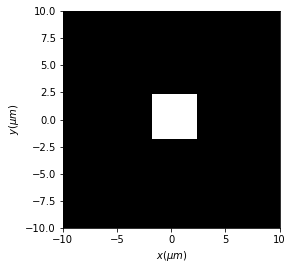
# slit
t0 = Scalar_mask_XY(x=x0, y=y0, wavelength=wavelength)
t0.square(r0=(0, 0), size=(4 * um, 4 * um), angle=0)
t0.draw()
plt.xlim(-10, 10)
plt.ylim(-10, 10)
u1 = u0 * t0
[11]:
u2 = u1.fft(remove0=False, new_field=True)
u2.draw(logarithm=1e-1)