6.2.2. Wave Propagation Method and BPM in 3D

WPM method is very fast. It is based on S. Schmidt et al., “Wave-optical modeling beyond the thin-element-approximation,” Opt. Express, vol. 24, no. 26, p. 30188, 2016.

[1]:

from diffractio import np, plt, sp, um, mm, degrees
from diffractio.scalar_fields_XYZ import Scalar_field_XYZ

from diffractio.scalar_masks_XY import Scalar_mask_XY
from diffractio.scalar_sources_XY import Scalar_source_XY
from diffractio.scalar_masks_XYZ import Scalar_mask_XYZ

6.2.2.1. Propagation at vacuum

[2]:

x = np.linspace(-50 * um, 50 * um, 256)
y = np.linspace(-50 * um, 50 * um, 256)
z = np.linspace(0, 500 * um, 256)
wavelength = .6 * um

[3]:

t0 = Scalar_mask_XY(x, y, wavelength)
t0.circle(r0=(0, 0), radius=45 * um, angle=0)

[4]:

u = Scalar_mask_XYZ(x, y, z, wavelength)
u.incident_field(u0=t0)

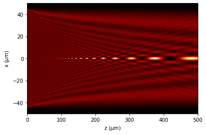
6.2.2.2. WPM

[5]:

%%time
u.clear_field()
u.WPM(verbose=True, has_edges=True)

Time = 6.44 s, time/loop = 25.17 ms
CPU times: user 5.88 s, sys: 730 ms, total: 6.61 s
Wall time: 6.58 s

[6]:

u.draw_XZ(y0=0, logarithm=False)

<Figure size 432x288 with 0 Axes>

../../../_images/source_tutorial_scalar_XYZ_wpm-bpm_3d_8_1.png

6.2.2.3. BPM

[9]:

%%time
u.clear_field()
u.BPM(verbose=True, has_edges=True)
u.draw_XZ(y0=0, logarithm=True);

CPU times: user 2.61 s, sys: 120 ms, total: 2.73 s
Wall time: 2.72 s

<Figure size 432x288 with 0 Axes>

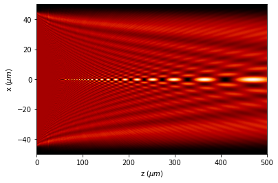
../../../_images/source_tutorial_scalar_XYZ_wpm-bpm_3d_10_2.png

At vacuum both techniques work fine.

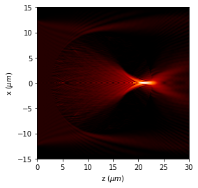
6.2.2.4. Diffraction by an sphere

WPM and BPM also allow propagation through a XYZ refraction index structure.

[11]:

x = np.linspace(-15 * um, 15 * um, 256)
y = np.linspace(-15 * um, 15 * um, 256)
z = np.linspace(0, 30 * um, 256)
wavelength = 0.6328 * um

[12]:

t0 = Scalar_mask_XY(x, y, wavelength)
t0.circle(r0=(0, 0), radius=12.5 * um, angle=0)

u0 = Scalar_source_XY(x, y, wavelength)
u0.plane_wave(A=1)

[13]:

u = Scalar_mask_XYZ(x, y, z, wavelength)
u.sphere(r0=(0, 0, 12.5), radius=10 * um, refractive_index=2, angles=(0, 0, 0))

[14]:

u.incident_field(u0=u0 * t0)

[15]:

# u.draw_refractive_index()

6.2.2.4.1. WPM

[16]:

%%time
u.clear_field()
u.WPM(verbose=True,has_edges=True)

Time = 7.79 s, time/loop = 30.42 ms
CPU times: user 7.86 s, sys: 117 ms, total: 7.97 s
Wall time: 7.93 s

[17]:

u.draw_XZ(y0=0, logarithm=True, scale='scaled')

<Figure size 432x288 with 0 Axes>

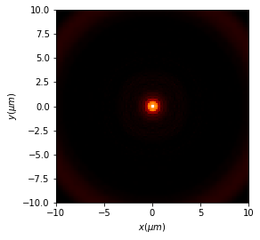
../../../_images/source_tutorial_scalar_XYZ_wpm-bpm_3d_20_1.png

[18]:

u2 = u.cut_resample([-10, 10], [-10, 10],
                    num_points=(128, 128, 128),
                    new_field=True)

[19]:

u2.draw_XY(z0=20.5, logarithm=True)

../../../_images/source_tutorial_scalar_XYZ_wpm-bpm_3d_22_0.png

[20]:

# u.draw_XYZ(logarithm=True)

6.2.2.4.2. BPM

[21]:

%%time
u.clear_field()
u.BPM(verbose=True,has_edges=True)

CPU times: user 2.8 s, sys: 140 ms, total: 2.94 s
Wall time: 2.98 s

[22]:

u.draw_XZ(y0=0, scale='scaled', logarithm=True)

<Figure size 432x288 with 0 Axes>

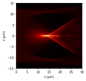
../../../_images/source_tutorial_scalar_XYZ_wpm-bpm_3d_26_1.png

In this case, the results are quite different. As the difference of refraction indexes is high, WPM produces better results.